Introduction

Diagnosing cardiac anomalies is a leading issue faced by medical researchers, and several methods have been used to estimate a heart’s “Cardiac Output”, that is, the volume of the ventricles, in both active (systolic) and resting (diastolic) states. The incentive behind doing so is to be able to effectively calculate the heart’s ejection fraction (EF), which is defined as the percentage of blood ejected from the left ventricle with each heartbeat. The ventricles’ volumes and the ejection fraction together are predictive of a number of heart diseases and hold much promise in early detection of cardiac anomalies. While multiple modalities can measure cardiac volumes and the subsequent ejection fraction, calculating them from Magnetic Resonance Imaging (MRIs) yields the best results. However, the current standard for the estimation of ventricle volumes is to have a cardiologist calculate them manually from MRIs in a rather time consuming process. Automating this process will allow doctors to diagnose heart conditions early/ better, and carries broad implications for advancing the science of heart disease treatment and therefore forms the inspiration of our project.

Problem Definition

Our aim is to automate the manual processing involved in determination of cardiac volumes by training a convolutional neural network(CNN) that can approximate the end-systolic/diastolic volume of the left ventricle using the same MRIs an expert would need. Our task is that of supervised regression, and the loss function used is mean square error (MSE) using convex L2 minimization.

Dataset

The data was sourced from the 2016 Data Science Bowl competition. The original dataset consisted of 4 channel (4ch), 2 channel (2ch) and multiple short axis (SAX) views for approximately 500 patients in the training set. However, the 4ch views were the most effective and usable form, as the ventricles are clearly visible in the coronal plane.
Post cleaning and filtering, we have 30 4-channel MRIs each for 480 patients, thus giving us a total of 14400 training images. The validation and test sets have 4ch MRIs for approximately 200 patients each. The images are in the DICOM (Digital Imaging and Communications in Medicine) format which also contained metadata such as age, sex, heart size for all the patients. The data occupied around 45 GB in total.

Survey

The three questions addressed by each paper are:
I. Main Idea
II. How’s the paper useful for our project?
III. What are the shortcomings, how do we improve upon them?

Paper- 1

I. Proposes first segmenting for the ROI and then cardiac output from MRI images as regression problem using CNNs.
II. Has used the same dataset as ours.
III. The combined approach for segmentation and cardiac output calculation might not work as well as a more modular approach.

Paper- 2, 3, 5

I. Explores ensemble learning, SVMs and Deep-Belief-Networks to achieve our project’s aim.
II. Advantages: good generalization, high accuracy for smaller amounts of training data and less variance can be incorporated.
III. These papers focus on small datasets with low variance and noise.

Paper- 4, 8, 11

I. Explains concepts of deep learning, tracking features across frames, active contours.
II. Our project uses the concepts mentioned above.
III. No shortcomings. These are seminal works, used as reference even today, post adaptation.

Paper-6

I. Proposes fully automated segmentation and tracking of the myocardium that can be used for measuring regional motion, deformation, as well as labelling and tracking specific regions of the heart.
II. Introduces potential transformations for segmentation of data.Also shows a way to relate images spatially and temporally.
III. Is done for 4D-MRI images, which is different from our dataset and cannot be used as is.

Paper-7

I. Proposes a method by which we can automatically segment the left ventricle from a 3D-MRI.
II. Explains how the data might be “unclean” due to variations in factors like blood flow, partial volume-effects etc.
III. Uses multi-model prior knowledge that is not applicable to our dataset.

Paper-9

I. Presents a segmentation approach that is robust and accurate on the short axis cardiac MRI.
II. Part of our dataset contains images that are short axis MRI images, thus making this approach important.
III. The ROI needs to be remedied with certain transformations to bring the ROI in the same form as the other images.

Paper-10

I. Proposes the use of a Deep-Belief-Network for detecting the ROI in the left ventricle of the heart.
II. Combining active contours with a DBN results in needing smaller datasets for training.
III. The method described needs manual initialization, which we avoid by using CNN.

Paper-12

I. Fast and robust implementation of a CNN to perform automated ventricle segmentation.
II. This model of segmentation of ventricles uses a single learning stage, and can leverage computational resources like GPUs at massive scales.
III. The models were trained on the Sunnybrook dataset, which is too small to create complex, powerful models.

Paper-13

I. A CNN is used for restoration of noisy or degraded images as opposed to traditional methods. Shows significant improvement in performance.
II. Useful because medical images received may be noisy or degraded and hence image-segmentation may not be possible.
III. Uses a feedforward network on every patch of the image hence slow. This will be solved by partially rarefying the weights[15].

Paper-14

I. Two networks in a recursive training architecture are used. One generates a preliminary boundary-map and another generates the final boundary-map.
II. Faster restoration of degraded images hence improving performance.
III. Computationally heavy, GPU acceleration will help.

Paper-15

I. Performs better than conventional statistical-shape models by utilizing random walks for segmentation.
II. Useful for accurate segmentation and shows better generalization.
III. The dataset doesn’t truly represent the actual data population which can be addressed by collecting more data.

Paper-16

I. Trains a neural net to learn augmentation and decide which augmentations best improves the classifiers.
II. Can potentially eliminate manual data-augmentation.
III. The automated augmentation might not result in improving the performance of the CNN.

Paper-17

I. Advocates using prior knowledge about the shape of the organ being analyzed and its location instead of only pixel-wise classifiers, when training CNNs.
II. Knowledge of anatomy of heart could be used to eliminate corrupted/misleading data.
III. No shortcomings.

Paper-18

I. Discusses image-processing and feature-extraction techniques when using a neural network to classify images.
II. Use feature-extraction and image pre-processing techniques.
III. Some techniques discussed are not applicable to our dataset.

Approach taken:

1. Proposed Method:

Our approach to solving the problem was to train a CNN that could potentially perform the task well enough in lieu of a trained cardiologist. In order to be able to do so, we first preprocessed the data to maximize the information that our features would be conveying to the CNN by using some traditional image processing techniques. We followed it up with the training of the CNN, and to justify the additional resources that are associated with it, we compared it to multiple other simpler, less compute and time intensive regressors.

2. Preprocessing:

The available data had a lot of inconsistencies such as varying sizes and orientations. Consequently, this is the task that we put most of our efforts and time in.
Since we wanted to create a CNN that was computationally efficient, but at the same time did not suffer from any biases and had a good sampling of the overall distribution, we restricted our input MRIs to those which had 4 channel views as the ventricles were seen most clearly in these images. It would be a reasonable assumption that a human expert would also choose a 4ch view over a 2ch or SAX view of the heart
All the input images were first resized to 256x256 pixels. The metadata was saved for later analyses. The region of interest (RoI) was near the center of the resized images and a 128x128 region around the RoI was extracted to keep only the relevant information and discard unnecessary data. The advantage of doing this is that the matrix formed after flattening and concatenating all the images will have only the relevant features, thus making the problem less underdetermined, leading to a better accuracy. This area was then resized to 64x64 to reduce computation time as smaller feature matrices reduce computation costs. Finally, a radial basis transfer function was applied on the extracted image to give a probability estimate for the final RoI in the cropped feature images.
For the regression methods described in the experiments section, the (64,64) 4ch images were flattened into (1x4096) vectors. Our input would therefore be an MxN matrix:
M ( #rows) = (4 ch images )*(# patients) = 30*480 = 14400
N (#columns) = 4096

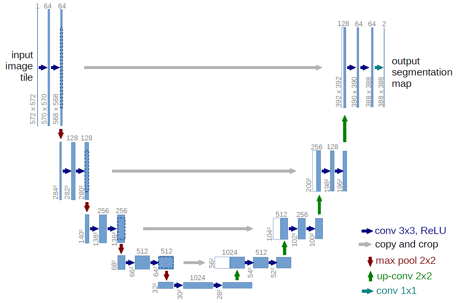
3. Architecture:

Our implemented CNN was a modified, simpler version of the U-Net architecture that has found much success in biological object recognition. It will consisted of convolutional, pooling and fully connected layers. Our intermediate activation functions are Rectified Linear Units (ReLUs) and the final is a sigmoid function.
Our model consisted of three convolutional layers, one flattening layer and two fully connected layers used as part of the CNN architecture. Each of three convolutional layers used a single convolved layer, max pooling, and Relu layer. The output of the third convolutional layer which was multidimensional tensor, which was converted to a one-dimensional tensor in the next layer which was the flattened layer. The output of the flattened layer was used to create the fully connected layer, which took all the inputs and used the standard z = wx + b operation on it. At the end Relu was used to add nonlinearity to it. The next layer was another fully connected layer that took the output of the last fully connected layer and performed the same operation, except this time Relu layer was not used. The output of the final layer was used as output of the CNN. Two separate convolutional neural nets used for end systolic and diastolic volume prediction. Learning rates ranging from 10-5 to 10-3, and batch sizes of 32,64,96,128 were tried, of which 10-4 ,32 worked best. The model took close to 800 epochs to converge.
The CNN optimized on the mean squared loss between the output of the last fully connected layer and the y_true data, when training. The entire architecture was implemented in TensorFlow.

4. Visualization:

We have made this website as part of our visualization. It includes an interactive scatterplot which displays the volume of LV along with the patient details sourced from the metadata available from the dicom images. We have compiled all the visualizations on a Tableau dashboard, published it on a server and have embedded it on this website.

Experiments, Evaluation and Results:

Our experiments ensured that the extra time and effort spent in designing and training the CNN was justified in terms of accuracy.​ Multiple toy models were implemented, thus giving us baseline estimates for different ML algorithms:
Linear Regression: The most basic regressor known to mankind, it is the most economical in terms of compute, with no parameters or hyper-parameters to tune, and is extremely simple to implement.​ It however, understandably had the lowest accuracy, but was extremely fast and simple to implement.
Support Vector Machine: Another popular ML algorithm, while SVMs aren't very quick, they provide good accuracies and when kernelized, can be extended to very high dimensions and highly non-linear mappings.
Single-layer Neural Network: We compared our program’s results against a single layer neural network’s to make sure that our approach justifies the additional time and compute required for a CNN as opposed to a vanilla neural net. The 1-layer NN acted as our baseline, minimum accuracy that we tuned the CNN to beat.
Random Forests: Random forests, which are an ensemble of different regression trees can be used for nonlinear multivariate regression. Each leaf contains a distribution for the continuous output variables. Just as with classification, random forests provide good accuracy and are fairly robust to biases in the dataset.
For the experiments, we used the standard cross-validation of 3 and worked with standard practices for hyperparameter tuning in the sklearn library. The MSE of the models were converted to accuracy percentages by using the true labels of our test data and taking its fraction.

Interactive Visualization:

List of Innovations:

1. Traditional image processing techniques were used to augment the machine learning methods to maximize the information content of our features, thus improving our models’ accuracies instead of simply collecting more data and making the process extremely compute and resource heavy.
2. We exploited a priori knowledge of the images to concentrate and enhance the parts of our images and reduce the effect and number of “outlier pixels” in it.
3. Our CNN is a more application-specific and computationally efficient version of the U Net.

Conclusion:

As expected, regular L2-minimizing linear regression performs least accurately. However, it serves as a good estimate as to for a minimum, required accuracy for any model that further develops. Using L1-minimization could possibly have provided a better fit and subsequent accuracy. We notice that the support vector regressor performs fairly well, which might imply that the data might be linearly separable once we perform a radial basis transformation. This isn’t surprising especially as we’ve used a radial basis smoothing on our input features. Random forests perform well, as expected, while the 1-layer neural network serves as a decent starting point for the CNN to improve upon.

Future Work

Further tuning of the hyperparameters will definitely improve the CNN’s accuracy, and is one of the most promising directions for future work. Another improvement would be to increase the number of layers and making the network deeper. This would introduce the possibility of bad generalization and overfitting, which could be combated with regularization techniques like drop-out, or techniques like early stopping.

References

[1] Estimating the volume of the left ventricle from MRI images using deep neural networks. Journal of Latex class files, Vol.14, No.8, August 2015. Fangzhou Liao, Xi Chen, Xiaolin Hu, Senior Member, IEEE and Sen Song

[2] Diagnosing Coronary Heart Disease Using Ensemble Machine Learning.(IJACSA) International Journal of Advanced Computer Science and Applications, Vol. 7, No. 10, 2016. Kathleen H. Miao , Julia H. Miao , and George J. Miao.

[3] Applying Machine Learning Methods in Diagnosing Heart Disease for Diabetic Patients. International Journal of Applied Information Systems (IJAIS) – ISSN : 2249-0868 Volume 3– No.7, August 2012. G. Parthiban and S.K.Srivatsa

[4] Y. LeCun, Y. Bengio, and G. Hinton, “Deep learning,” Nature, vol. 521, no. 7553, pp. 436–444, May 2015.

[5] T. A. Ngo and G. Carneiro, “Left ventricle segmentation from cardiac MRI combining level set methods with deep belief networks,” in Proceedings of International Conference on Image Processing, Sep. 2013, pp. 695–699.

[6] M. Lorenzo-Valds, G. I. Sanchez-Ortiz, R. Mohiaddin, and D. Rueckert, “Atlas-Based Segmentation and Tracking of 3D Cardiac MR Images Using Non-rigid Registration,” in Proceedings of International Conference on Medical Image Computing and Computer Assisted Intervention. Springer Berlin Heidelberg, Sep. 2002, pp. 642–650.

[7] M. R. Kaus, J. von Berg, J. Weese, W. Niessen, and V. Pekar, “Automated segmentation of the left ventricle in cardiac MRI,” Medical Image Analysis, vol. 8, no. 3, pp. 245–254, 2004.

[8]P. Viola and M. Jones, “Rapid object detection using a boosted cascade of simple features,” in Proceedings of IEEE Conference on Computer Vision and Pattern Recognition, vol. 1. IEEE, 2001, pp. I–511.

[9]H. Hu, H. Liu, Z. Gao, and L. Huang, “Hybrid segmentation of left ventricle in cardiac MRI using gaussian mixture model and region restricted dynamic programming,” Magnetic Resonance Imaging, vol. 31, no. 4, pp. 575–584, May 2013.

[10]T. A. Ngo, Z. Lu, and G. Carneiro, “Combining deep learning and level set for the automated segmentation of the left ventricle of the heart from cardiac cine magnetic resonance,” Medical Image Analysis, vol. 35, pp. 159–171, Jan. 2017.

[11] M. Kass, A. Witkin, and D. Terzopoulos, “Snakes: Active contour models,” International Journal of Computer Vision, vol. 1, no. 4, pp. 321–331, 1987.

[12] P. V. Tran, “A Fully Convolutional Neural Network for Cardiac Segmentation in Short-Axis MRI,” arXiv:1604.00494 [cs], Apr. 2016.

[13] V. Jain, J. F. Murray, F. Roth, S. Turaga, V. Zhigulin, K. L. Briggman, M. N. Helmstaedter, W. Denk, and H. S. Seung, “Supervised Learning of Image Restoration with Convolutional Networks,” in Proceedings of IEEE International Conference on Computer Vision, Oct. 2007, pp. 1 – 8.

[14] K. Lee, A. Zlateski, V. Ashwin, and H. S. Seung, “Recursive Training of 2D-3D Convolutional Networks for Neuronal Boundary Prediction,” in Advances in Neural Information Processing Systems, 2015, pp. 3573–3581.

[15] A. Eslami, A. Karamalis, A. Katouzian, and N. Navab, “Segmentation by retrieval with guided random walks: Application to left ventricle segmentation in MRI,” Medical Image Analysis, vol. 17, no. 2, pp. 236–253, Feb. 2013.

[16] Jason Wang, Luis Perez, “The Effectiveness of Data Augmentation in Image Classification using Deep Learning”, ArXiv e-prints, Dec. 2017.

[17] Ozan Oktay, Enzo Ferrante, Konstantinos Kamnitsas, Mattias Heinrich, Wenjia Bai, Jose Caballero, Stuart Cook, Antonio de Marvao, Timothy Dawes, Declan O’Regan, Bernhard Kainz, Ben Glocker, and Daniel Rueckert, “Anatomically Constrained Neural Networks (ACNN): Application to Cardiac Image Enhancement and Segmentation”, IEEE Transactions on Medical Imaging, AUG 2017.

[18] Elalfi A., Eisa M. and Ahmed H, “Artificial neural networks in medical images for diagnosis heart valve diseases”, International. Journal of computer science issues, 2013.